I’ve spend quite some time with PCA for the last couple of months and I thought I would share some of my notes on this subject. I must caution that this is one of the longest post I’ve done. But I find the subject very interesting as it has a lot of potential in the asset allocation process.
PCA stands for principal component analysis and it is a dimensionality reduction procedure to simpify your dataset. According to Wikipedia, “PCA is a mathematical procedure that uses orthogonal transformation to convert a set of observations of possibly correlated variables into a set of values of linearly uncorrelated variables called principal components.” It is designed in a way such that each successive principal components explains a decreasing amount of variation in your dataset. Below is a screeplot of the percentage variance explained by each factor on a four asset class universe.

PCA is done via an eigen decomposition on a square matrix which in finance is ether a covariance matrix or a correlation matrix of asset returns. Through eigen decomposition, we will get eigenvectors (loadings) and eigenvalues. Each eigenvalue, which is the variance of that factor, is associated with an eigenvector. The following equation relates both the eigenvectors and eigenvalues.

The eigen vector E of a square matrix A equals to an eigenvalue (lambda) multiplied by the eigenvector. While I must confess I was bewildered towards the potential application of such values and vectors at school, it does come to make more sense when you place it in to financial context.
In asset allocation, PCA can be used to decompose a matrix of return into statistical factors. These latent factors usually represent unobservable risk factors that are imbedded inside asset classes. Therefore allocating across these may improve one’s portfolio diversification.
The loadings (eigenvectors) of a PCA decomposition can be treated as principal factor weights. Another words, they represents asset weights towards each principal component portfolio. The total number of principal portfolios equals to the number of principal components. Not surprisingly, the variance of each principal portfolio is its corresponding eigenvalue. Note that the loadings are designed to have values ranging from +1 to -1 meaning short sales are entirely possible.
Since I am not a math major, I don’t really understand any math equations until I actually see it being programmed out. Lets get our hands dirty with some data:
rm(list=ls())
require(RCurl)
sit = getURLContent('https://github.com/systematicinvestor/SIT/raw/master/sit.gz', binary=TRUE, followlocation = TRUE, ssl.verifypeer = FALSE)

con = gzcon(rawConnection(sit, 'rb'))
source(con)
close(con)
load.packages('quantmod')

data <- new.env()

tickers<-spl("VBMFX,VTSMX,VGTSX,VGSIX")
getSymbols(tickers, src = 'yahoo', from = '1980-01-01', env = data, auto.assign = T)
for(i in ls(data)) data[[i]] = adjustOHLC(data[[i]], use.Adjusted=T)

bt.prep(data, align='remove.na', dates='1990::2013')

prices<-data$prices
ret<-na.omit(prices/mlag(prices) - 1)
To calculate return we can simply

This can be represented by in R by
weight<-matrix(1/ncol(ret),nrow=1,ncol=ncol(ret))
p.ret<-(weight) %*% t(ret)
Note that if R is a multi-row matrix return series, you will actually get back a vector of return series with the same number of rows as R. This is simply the portfolio return series, assuming daily rebalancing.
There are like 3 different way of doing a PCA in R. I will show a foundational way and a functionalized way of doing it. Such two-step process will help see what’s going on under the hood.
#PCA Foundational
demean = scale(coredata(ret), center=TRUE, scale=FALSE)
covm<-cov(demean)
evec<-eigen(cov(demean), symmetric=TRUE)$vector[] #eigen vectors
eval<-eigen(cov(demean), symmetric=TRUE)$values #eigen values
#PCA Functional
pca<-prcomp(ret,cor=F)
evec<-pca$rotation[] #eigen vectors
eval <- pca$sdev^2 #eigen values
The foundational way uses the build in “eigen” function to extract the eigenvectors and eigenvalues. This way requires that you demean (scale function) the data before calculating the covariance matrix. The return values are stored in a R list data structure. On the other hand, the functional PCA just takes in an return series vector and it does the rest.
After calculating the eigenvector, eigenvalues, and the covariance matrix, the following equation will hold true:

In the above equation, E and lambda, again, are the eigenvector and eigenvalues respectively. Sigma represents the demeaded covariance matrix. In R, this can be computed by:
diag(t(evec) %*% covm %*% evec) #reverse calculate eigenvalues
Now we have all the components to calculate principal portfolios. These return series are simply the latent factors that are embedded inside asset classes. Each asset class are exposed to each factor pretty consistently through time which may help further understand the inherent risk structure. To calculate the principal component portfolios, we will use the following formula:

This equation is very intuitive as just like earlier, the eigenvectors are “weights,” therefore applying it to the returns will yield the N different principal portfolio return streams. In R:
inv.evec<-solve(evec) #inverse of eigenvector
pc.port<-inv.evec %*% t(ret)

In Meucci’s paper “Managing Diversification”, he showed that with the following formula one can convert a vector of weights from the asset space to the principal component space. More specifically, given a vector of asset weights, one could now show the exposure to each principal component.

Next I would like to show how from the above equation one will be able to calculate the exposure of traditional portfolio optimization weights to each principal component factors. I will be using the same universe of assets and applying Minimum Variance, Risk Parity, Max Diversification, Equal Risk Contribution, Equal Weight, and David Varadi’s et al Minimum Correlation Algorithm (mincorr2).

As you can see, risk base portfolio optimization in the traditional asset space leads to excessive exposure towards the interest rate factor (bonds). The general equity risk factor (factor 1) accounts for the second largest concentration. Prudent investors looking at this chart will immediately notice the diversification potential if one were to allocate to factors 2 and 3.
In R, the principal component exposure equation can be calculated as follows:
factor.exposure<-inv.evec %*% t(weight)
Through simple algebra, one can convert back and forth between the asset space and the principal space easily. In the following example, I am reconstructing using equal weights.
pc.port<-as.xts(t(pc.port))  #correct dimension of principal portfolio returns
p.ret1<-t(factor.exposure) %*%  t(pc.port)
If you are following along, you will notice that the equity curves derived from the variables “p.ret” and “p.ret1” are identical. This confirms that we have correctly converted back to the asset space.
Next, to calculate the variance contribution due to the N-the principal component we can simply:

A neat aspect is that from the above equation, we can arrive at the portfolio variance in the asset space with the following equation (sum because PCs are uncorrelated):
The following R code confirms that their variance are the same in the PC space and the asset space.
sum((factor.exposure^2)*eval) #variance concentration from PCA
apply(p.ret,2,var) #portfolio risk from equal weight
With this as proof, one can actually reformulate the minimum variance portfolio from the principal space. We know that portfolio variance can be calculated according to the following formula
Just to repeat, we know that given a set of asset weights we can calculate our exposure to each principal factor using:
![]() Isolating asset weights, substituting and then simplifying:
Isolating asset weights, substituting and then simplifying:
Since we know that
Then portfolio variance is simply
This is intuitive as since the correlation between principal portfolios are zero, the covariance are all zero too. What is left behind are the variances of the eigen portfolios. Minimizing the above and converting the weights back to asset space should give you equivalent weights from a MVO. While I understand that there is no practicality in the above steps as it adds complexity and computing power, I just wanted to illustrate that these two spaces are tied together in many aspects.
This post is going to get out of hands if I don’t stop. As you can see PCA is a very interesting technique, it allows you to access latent factors and how they interact with the asset space. I hope curious readers can go on exploring more and post below if you find any interesting things you stumble across.
Thanks for reading,
Mike

Mike, great post. I also find factors an interesting topic. Is it possible to share the code you used to calculate the optimized exposures? Would love to learn.
Also, what do you think of macro factors as for example http://www.callan.com/research/download/?file=papers%2Ffree%2F586.pdf
Thank you.
sorry Raf, didn’t see this comment till now. must’ve slipped through..
So given to get the optimized exposures, you will need to do the following:
1. get the daily return streams (assume they are stored in “ret” variable)
2. do a PCA decomposition on those return streams:
pca<-prcomp(ret,cor=F)
3. get the loadings
loadings<-pca$rotation[]
4. Invert the matrix
inv.evec<-solve(loadings)
5. with inverted eigenvector, you can get a set of weights, say from min.var can do the following:
inv.evec %*% t(weight)
That will get you the PCA factor exposures given the weights.
Hello,
Is it possible to share the code to replicate the graphics?
Regards
hello barbaros:
the bar charts are generated from R using “barplot” command. See: http://www.statmethods.net/graphs/bar.html
the 4 time series factor chart is generated via R’s lattice package function: xyplot
xyplot takes a index, in my case xts time object
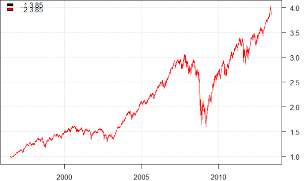
The last chart where I plot the red equity line is from SIT packages command “plota.matplot()”
“As you can see, risk base portfolio optimization in the traditional asset space leads to excessive exposure towards the interest rate factor (bonds).”
I see an exposure to PC4 but how can you tell it is the interest rate ? I thought principal components were synthetic variables that were linear combination of existing variables ?
If you roll the loadings of PC4 over time, you will find that it has a high positive exposure to the bonds relative to all the other factors.
hey I am currently doing a project on PCA. I used your r codes and I got till inverse eigen vectors. I couldnt figure out why this
factor.exposure<-inv.evec %*% t(weight)
R throws an error as weight not defined .
Can you pls help me on this man?
U need a wight vector to find exposures to the factors, else it won’t work.
Thank you very much for this post! Its been a while since I did hard mathematics at Uni and this was crisp and well summarized version of PCA in a financial context!
Hello Mike. Very interesting article. Unfortunately there are a few pictures missing now. How can I access them? separately, what is the cor=F parameter in prcomp… not documented in the function description. Thanks
great article, if anyone wished to calculate the estimated covariance matrix based on the PCs chosen, then regress the original data set wrt to the PCs and use the regression coefficients (B) and residual errors such as B*np.cov(PCs)*B’ + diagonal of errors. If you use all PCs the estimated covar is the same as original data set covar. This is useful when it comes to portfolio optimization when you need to input you covar matrix.