The Man Who Solved the Market – Notes

When it comes to the world’s most secretive hedge fund any content is worthwhile to read. I finished the book is 3 days and had to re-read a couple more chapters to ensure I fully absorbed the couple nuggets in there. I would recommend this book to everyone!

The mystery behind how Simons discovered the “truth” is shrouded in mystery. Even googling about what they traded doesn’t yield many answers. This new book by Gregory Zuckerman was an eye opener. It revealed how Renaissance came to be including Simons early struggles.

One of the surprising things I’ve learned was that Simons was actually the money guy. Though he did trade and built up the business in the early years, he wasn’t the main guy leading the research breakthroughs. Instead Simons seem to be running side gigs like investing in start ups back in the day. People like Ax, Berlekamp, Carmona, Laufer, Mercer, and Brown were the main brains behind all the models.

Now to the trading models. Even though the author isn’t trained in finance, I really think he did a decent job explaining some of the broad concepts utilized by Renaissance in the early days. Before 1988 (right before Carmona joined), Renaissance was a typical CTA / point and click trading firm. They utilized breakout models/linear regression (page 83). What changed around that time was both Carmona and Laufer started to data mine for trading patterns as oppose to hand crafting them. This especially stood out for me personally as about a year ago I started to conduct research via data mining. As Renaissance thrived through the 90s, more than 50% of their models were data mined. (page 203) Their reasoning resonated with me a lot. “Recurring patterns without apparent logic to explain them had an added bonus: They were less likely to be discovered and adopted by rivals…”

Additional interesting tidbit:

• “Laufer’s work also showed that, if markets moved higher late in a day, it often paid to buy futures contracts just before the close of trading and dump them at the markets opening the next day.” Isn’t this the overnight premium hes talking about for equity futures? Sure sounds like it…. (page 144)
• On the subject of managing models, Laufer insisted on a single model as oppose to multiple models. (page 142) Presented with many different signals, they built a trade selection algorithm that further determines which trades to take. Strategies that did well will automatically without human intervention get allocated more money.(page 144)
• Started out trading end of day and slowly breaking down in to 2 sessions per day. Simons then suggested going down to 5 minute bars. (page 143)
• “Did the 188th five-minute bar in cocoa future market regularly fall on days investors got nervous, while bar 199 rebounded?” page(143) Looked at intraday seasonality and conditional signals. Edge layered over edge to increase probability of being right.
• Mercer and Brown took over Keplers Stat arb operation. Soon stock trading pnl was greater than futures trading.

While I am sure today’s Renaissance is far from what the booked described, the broad concepts like data mining, alternative data collection, and stat arb all play a role in their continued success in some form or fashion. Please let me know if I’ve missed anything interesting. Of course, I may have interpreted it entirely wrong. Please leave a comment below!

 

Bibliography:

Zuckerman, Gregory. The Man Who Solved the Market. Portfolio/Penguin, 2019.

Queue Position Simulation

First off, Happy Thanksgiving! If time permits in the coming months I’d like to explore more on how I look at High Frequency (HF) data. Hopefully along the way I can spark some new discussion and improve on my thought process.

HFT strategy “simulation” is no easy task. I am referring to this as an simulation because its purely an approximation of how a strategy would have performed given a set of execution assumptions the researcher made beforehand. Should the assumptions change, the results would also change (significantly).

In my line of work, the edge we are seeking are generally less than a tick (futures). To make this even worth while, the constraints are that costs must be low AND we need to trade a lot. This may sound foreign to most of my readers as their time frames are generally much longer (days, weeks, even months). But at the end of the day, how much money we make is a simple function of our alpha * number of times we trade.

In HFT, execution is king. You can be right where the market moves the next tick but if you can’t get a fill, you are not making any money. Therefore it is paramount that when we conduct HF simulations, we make accurate execution assumptions.

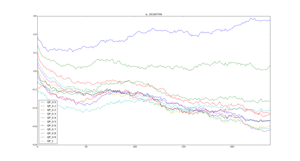
Queue position, this is something that is worth a lot. Being first in line and getting a fill is like owning a call option in my world (where the premium is exchange fees per contract). The worst that can happen is you scratch assuming you are not the slowest one and there are people behind you. The image below is an analysis done on the expected edge you’d get N-events out (x-axis) assuming you are in various spots within the fifo queue. (QP_0 = first in line, QP_0.1 = 10th in line if there was 100 qty). As you can see, the further behind in line you are, the more you are going to be exposed to toxic flow, fancy word for informed traders.

 

How does one take this in to account when you simulate a strategy? When you place a limit order on the bid, how do you know when you will be filled? This depends on 2 factors, your place in line and trade flow. As time progresses there will be people who add orders to the fifo queue, people who cancel orders and people who take liquidity (trade). These actions are something one needs to keep track of tick by tick (or packet by packet) during a simulation. While most people assume tick data is the most fine grain dataset one can have in performing such simulations there actually exists packet data. Tick data simply gives you an aggregated snapshot of what an orderbook looks like – best bid, best offer, bid qty, ask qty (this is known as Market by price). Packet data on the other hand contains all the actions taking by all the market participants. This includes, trade matches and order submissions. This feed is also know as Market by order and its up to the market participant to build and maintain their own orderbook. Using packet data for simulation would be the most optimal as you will know exactly where you are in line.

When you only have tick data, the only way to conduct these type of simulations would be to make assumptions. Here is a simple example. When you place a limit buy on the bid you are going to be last in line. You keep track of two variables, qty_in_front and qty_behind. Additions are straight-forward. Just add them to qty_behind. Cancels are a little more tricky because you don’t know whether its coming from people in front of you or people behind. A work around is to have something I call a reduce ratio. Its can take a value between 0 and 1 and it controls the percentage that is cancelling in front of you. For example, in ES simulations, I would set this to around 0.1  ie when there is a total of 100 qty cancells, I’d assume 10 happens in front of me and 90 happens behind me. There are edge cases but I’ll leave the reader to figure it out themselves. This is just a way, not the only way, of going about simulating a fifo queue. More complicated ways include dynamically adjusting the reducing ratio as you approach the front of the queue.

How do you guys go about this? I’d love to hear.

 

Constant Maturity Data

I’ve been asked multiple times why/when I use constantly maturity data for research and modelling. I thought I’d cover it here on my blog since its been a while. I hope to post more in the coming months/future as it has been a good way for me to organize my thoughts and share what I’ve been working on.

Constant maturity (CM) data is a way of stitching together non-continuous time series just like the back adjusted method. It is used heavily in derivative modelling due to the short-term time span a derivative (options, futures, etc) is listed/traded.

What is it and how is it used?

The CM methodology is essentially holding time constant. Various derivative contracts behave differently as time approach expiration so researchers developed this method to account for that and study the statistical properties through time.

I’ll provide a couple of usages.

In options trading, we know that time is one of the major factors that affect the price of an option as it approaches expiry. Options that expire further out in time are more expensive than options that expire closer to today. The reason for this is due to the implied volatility (IV). Researchers who want to study IV across time but not take the expiration affect in to account needs to hold time constant. For example, the study of how IV changes as a stock option approach earning announcements.

In futures, the CM methodology can be used to model the covariance matrices for risk analysis. For example, if you are trading futures under the same root (Crude) across various expirations, this method has shown to be rather useful is managing portfolio level risk.

For cash, the standout examples are the recent proliferation of the volatility ETPs. Most of these products are structured in a way to maintain a constant exposure to a given DTE. They will buy/sell calendar spread futures daily to rebalance their existing position.

How do you calculate it?

I’ve come across multiple ways of doing this. I will show you the most basic way and readers can test out which suit them best. The method I’ve used in the past is a simple linear interpolation given points. So assuming you are calculating IV for 30 days but you only have IV for a 20 and 40 DTE ATM option the equation is:

cm.pt = ( (target.dte – dte.front) * price_1 + (dte.back – target.dte) * price_2 ) / (dte.back – dte.front)

Here target DTE is the expiration you want to calculate. DTE.front should be < DTE.back as the front signifies it expires before the back. This is not the only way; there are other ways just like non-linear interpolation, etc. Carol Alexanders books provide more examples and much better explanations than I ever can!

Hope this helps!

Mike

Vertical Skew IV

Vertical Skew is the shape of the implied volatility (IV) term structure for a single options chain maturity. There is also something called a horizontal skew which is the IV across maturities. The movement of the vertical skew structure has been of interest to me recently when analyzing some of my option positions.

I had a long put butterfly position on with center short strikes 20 points below market. At trade initiation my greeks were as follows: Delta: -56, Gamma: -1.04, Theta: 117.9, Vega -343.8. This is generally what you’d expect for a short vol position. Delta is slightly negative due to the fly being bearishly positioned. My expectation was that for any decline in the markets you’d expect reduced pnl decline due to the fact that the delta will partially offset vega. As it turns out this is not the case, my position actually gained money on a price decline which was opposite to what my greeks are telling me. To understand we must look at IV Skew.

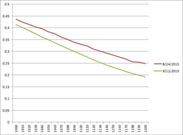
Below are the IVs for RUT September 2015 expiration put options. I specifically picked this period to illustrate the transition from high vol to low vol environment. If you look closely, you will notice that the green line is steeper than the red line. The second graph is the difference between the two line – its increasing. As we go from OTM options to ITM options, the rate of change of IV increases. Another words in our graph, ITM options (right side) will decline more in value (steepens) then OTM and ATM option when IV drops (vice versa for increases in IV – flatten). This phenomenon is not captured by the Black Scholes model as it assumes fixed volatility during the lifetime of the option.

 

Now how does this help me understand what happened to my position? Well, my right wing (highest strike) put option within my fly is an ITM option. When I was analyzing my position, I assumed that the long put wings of my fly had equal pnl contribution but that’s not the case. My right wing benefited the most from a given IV increase which means the overall negative effect of vega was over-estimated. In fact it may (and I am not 100% sure) be that both delta and vega was working in my favor assuming that the pnl contribution of the long wings was greater than the losses incurred from the short center strikes of my fly. Armed with this information, I think people can incorporate this in to their adjustments and maybe create some ways to exploit this. Open to any ideas!

Pretty cool eh?

Automated Trading System – Internal Order Matching

Most automated trading systems (ATS) are built such that there are little to no interactions between component models. This is limiting. Here I am referring to a trading system as the overarching architecture that houses multiple individual models.

Without interactions, each model is operating within an environment that it is preconceived in. For example, mean reversion can happen in different time/event frequencies. A model that is parameterized to take advantage on certain frequency will not have knowledge of others.

One component within an ATS that is rather complicated to architect is the order management system. The OMS is the component that handles all order requests generated by the prediction models. It must always be aware of outstanding orders (limit/market, etc), partial fills, and proper handling of rejects,etc. Now the complexity is increased when a portfolio of prediction models all generate an order for a given tick. (Which should be processed first?)

The general rule of thumb in dealing with this is to aggregate all orders by asset to reduce transaction costs. If there are a mix of long/shorts, the net will be the final order quantity. When it is filled, simply dis-aggregate them back in to component fills to the respective models (internal matching). The annoying part, in my opinion, is when you introduce multiple order types. For example, Limit and Market orders. How would one architect the OMS to handle both? Hmm.. This goes back to the debate of the degree of coupling between the strategy and the OMS itself….

CRSM Code

The code below represents the CRSM algorithm. It is adopted to the SIT framework. I have refactored the code so that its is easier for the user to use and understand.

I would like to once again thank you David Varadi for his tireless effort in guiding me along this past year. My gratitude also goes out to Adam Butler and BPG Associates for their support  all along the way.

Download Code: here

Thanks,

Mike

Shiny Market Dashboard

I’ve been asked multiple times regarding code for the dashboard so thought I’d release it. I coded the whole thing in one night last year so it’s not the best and most efficient, buts it’s a good framework to get your own stuff up and running. It’s long, north of 700 lines of code.

https://www.dropbox.com/sh/rxc8l4xnct5bcci/AABvTD2iJjC6wicLed3q9Qr3a

On another note, I’ve recently graduated from University and am excited to be moving to Chicago in a month for work. I am looking forward to the exciting opportunity. Also I will be releasing my graduating thesis in the coming weeks on RSO optimization. David Varadi has been my thesis advisor and mentor and I want to thank him for that!

Mike

Natural Language Processing

I’ve recently updated some matlab code about machine learning on to github. Today I’ll be adding to that with some Natural Language Processing (NLP) Code. The main concepts we covered in class were ngram modelling which is a markovian process. This means that future states or values have a conditional dependence on the past values. In NLP this concept is utilized via training n gram probabilities models on given texts. For example, if we specify N to equal to 3, then each word in a given sentence depends on the last two words.

So the equation for conditional probability is given by:

Extending this to multiple sequential events, this is generalized to be (chain rule)

 

This above equation is very useful for modelling sequential stuff like sentences. Extension to these concepts to finance are utilized heavily in hidden Markov models that attempts to model states in various markets.  I hope the interested reader comment below for other interesting applications.

The last topic we are covering is class is computer vision. As of now, topics like image noise reduction via Gaussian filtering, edge detection, segmentation are being covered. I will post more about them in the future.

Code Link

Cheers,

Mike

Artificial Intelligence

Artificial intelligence surrounds much of our lives. The aim of this branch of computer science is to build intelligent machines that is able to operate as individuals; much like humans. I am sure most of us have watched the Terminator movie series and questioned to what extent will our own society converge to that in the movie. While that may sound preposterous, much of what automated system developers do revolves around building adaptive systems that react to changes in markets. Inspired by a course I am taking at school right now, I would like to use this post as a general fundamental intro to AI.

If you ask people what intelligence is, most will initially find it hard to wrap words around the idea. We just know what it is and our gut tells us we, humans, are the pinnacle of what defines intelligence. But fact is, intelligence encompasses so much. According to the first sentence in wikipedia, there are ten different ways to define it.

“Intelligence has been defined in many different ways including logic, abstract thought, understanding, self-awareness, communication, learning, having emotional knowledge, retaining, planning, and problem solving.” -Wikipedia

Since it encompasses so much it is not easy to define it in a single sentence. What can be said is that intelligence relates to one’s ability to problem solve, reason, perceive relationships, and learn.

Now that I’ve offered a sense of what intelligence means, what, on the other hand, is artificial intelligence? Artificial intelligence is the field of designing machines that is capable of intelligent behavior; machines that is able to reason; machines that is able to learn. More precisely, the definition of AI can be organized in to four different sections:

• Thinking Humanly
• Thinking Rationally
• Acting Humanly
• Acting Rationally

The first two relates to thoughts processes while the last two relates to behavior. Thinking humanly revolves around whether the entity in question is able think and have a mind of its own. This is essentially making decision, learning and  problem solving. Acting humanly is whether a machine is able to process and communicate language, store information or knowledge and act based on what it knows and learn to adapt based on new information. These set of required traits are formulated based on the famous Turing Test which examines if a machine is able to act like a human through answering questions asked by anther human being. The machine passes the test if the person asking the question isn’t able to determine if its a machine or human. Thinking rationally closely incorporates the study of logic and logical reasoning. It was first introduced by Aristotle who attempted to provide a systematic way of inferring a proposition based on a given premise. An famous example would be “Socrates is a man; all man are mortal; therefore, Socrates is mortal.” Lastly, acting rationally is the idea of choosing the most suitable behavior that produces the best expected outcome. Another word one is rational if given all its knowledge and experience, selects the action that maximizes their own performance measure/utility.

Agents

When studying AI, the term agent is used to represent an entity/model that interacts with the environment. More precisely, an agent perceives the environment through its sensors and employ actions through actuators. Comparing this to humans, imagine sensors as eyes/ears and actuators as arms and legs. The sensors will at each time step take inputs, called percepts, which are than processed by the agent program. The agent program then passes the inputs in to an agent function. The agent function maps inputs to correct outputs (actions) which are then sent via the agent program to the actuators. This agent based framework closely relates to automated trading systems. The environment is the market and the changing prices at each time interval. The agent program would be our trading system which takes in daily price information and pipes it into the agent function, or the logic of the trading system. For example, todays new price is updated which is passed in to the trading logic. The logic specifies that if the current price is $10, it will sell. The sell action is passed back to the environment as a sell order.

The above example is a very basic type of agent known as the simple reflex agent. This type of agent only makes decision solely on the current percept (price). It doesn’t have a memory of the previous states. A more complex agent known as the model based reflex agent is one in which it has memory of the past, known as its own percept sequence. Also this agent has an internal understanding of how the environment works which is detailed in its own model. This model of the world takes inputs and identify the state it is in. Given the state, the model forecasts what the likely environment will be like in the next time step. Proper action is then recommended and executed via actuators. (Think of markov models)  So far, the agents I’ve introduced largely reflect that of a function that take input and spits out a output. To make things more humanly, the next agent I will introduce is called a goal based agent. This is similar to how given our current circumstances, we aim to maximize out objective function. The objective function can be money or anything that makes us happy. More concretely, the goal based agent is an extension of the model based reflex agent but it assigns a score for each recommended action. The agent will choose the one that maximizes its own objective function.

The reader will most likely ask how this knowledge helps them make money in the markets. What I can say is that finance is enter a brave new world where together with technology is transforming how money is being made in the markets. Having a understanding in finance and statistics in my opinion is not enough. Those are the areas where your competitors are already fishing (mostly). Knowledge in subject areas like AI, speech recognition, natural language processing, machine learning, and computer vision (just to name a few) will allow you to be more creative in design. I urge the curious minds to explore the unexplored!

Beyond Pairs

Writing rather prolifically this past week. Last week was the end of my midterms (for now!) and continuation of job search and preparing for my final 5 weeks of university.(!) I hope my readers are finding my posts interesting and enlightening.

As mentioned in an earlier post on statistical arbitrage, the interesting aspect of it comes when we consider multi leg portfolios. To construct a multi-leg portfolio, the traditional way to do it would be to employ a multivariate linear regression (factor model). The intuition behind this is that we are trying to estimate a fair value for an asset using various predictors or independent variables. For example, we know that the S&P 500 is composed of stocks from various sectors. Therefore, an intuitive way is to derive a fair value for S&P 500 using the 9 different sector Spdrs by the following equation:

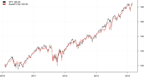
The residual return that is left over, “alpha”, is considered to be neutral (uncorrelated) against the industry sectors. With this framework, we now can essentially make ourselves neutral to any factors we want. For example, we have access to a wide variety of ETFs that mimic underlying asset class movements. If we want to be neutral to interest rates, credit risk, and volatility, we can employ ETFs: TLT, HYG, and VXX respectively. Below is a chart demonstrating this, showing the estimated fair value of SPY relative to the actual ETF:

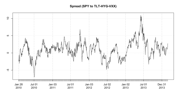
Below is the spread that can be traded via long short on each leg:

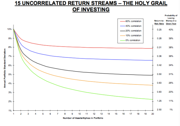
The concept of being able to control the factors we are exposed to is very appealing as it allows us to potential shy away from turbulent events that transpire from specific assets. Not only that, these uncorrelated return streams when combined in to a portfolio allows significant risk reduction. As Dalio said, the ability to combine 15 uncorrelated return streams allows us to effectively reduce 80% of risk. (Chart below) Interestingly, from my understanding of what Bridgewater does, I am pretty confident they are employing spread trading too, but purely from a fundamental way. For example, how does a set of asset classes react to the movements of economic indicators? From there they construct synthetic spreads to trade off of these relationships.

Below is the code that generated the data for this post:

spread.analysis<-function(data, y.symbol, x.symbol, lookback=250){
    y = data$prices[,y.symbol]
    x = data$prices[,x.symbol]
    lm.holder<-list()
    fv = NA * data$prices[,1]
    colnames(fv) = c('FairValue')

    for( i in (lookback+1):nrow(data$prices) ){
        cat(i,'\n')
        hist.y = y[(i-lookback):i, y.symbol]
        hist.x = x[(i-lookback):i, x.symbol]
        lm.r = lm(hist.y ~ hist.x)
        lm.holder[[i]] = lm.r
        fv[i,] = lm.r$coefficients[1] + sum(lm.r$coefficients[-1] * x[i,])
    }
    mat = merge( x,y,fv )
    return( list( mat = mat, fv = fv, reg.model = lm.holder ) )
}

Also here are some links I’ve found to be very informative.

• Mean Reversion – Quantivity
• Wonder of Residuals – Quantivity
• Ed Thorp Article Series On Stat Arb (Sick stuff here!!!)
• Market Neutrality (Quantum Financier)
• High Frequency & Dynamic Pairs Trading ( Energy Stocks )-Quantivity Paper Feed
• Gekko Quants 3 Part Series on Stat Arb ( Part I, II, III )
• Treasury Term Structure Arbitrage – Equametrics

The paper on high frequency statistical arbitrage is rather a relevant one as it relates to my previous blog posts on energy related pairs trading. Essentially, the author goes on to construct a meta algorithm for ranking pairs to trade. This meta-algorithm is composed of correlation coefficient, minimum square distance of normalized price series, and a co-integration test value. I don’t have intraday (paper used 15 min bars) equities data nor do I have the infrastructure to test it but the idea resonates with me from my research in top N momentum systems. A lot of ways to improve.